Dummy variables
Dummy variables are used when we are hoping to convert a categorical feature into a quantitative one. Remember that we have two types of categorical features: nominal and ordinal. Ordinal features have natural order among them, while nominal data does not.
Encoding qualitative (nominal) data using separate columns is called making dummy variables, and it works by turning each unique category of a nominal column into its own column that is either true or false.
For example, if we had a column for someone’s college major and we wished to plug that information into linear or logistic regression, we couldn’t because they only take in numbers! So, for each row, we had new columns that represent the single nominal column. In this case, we have four unique majors: computer science, engineering, business, and literature. We end up with three new columns (we omit computer science as it is not necessary and can be inferred if all of the other three majors are 0). Figure 11.7 shows us an example:
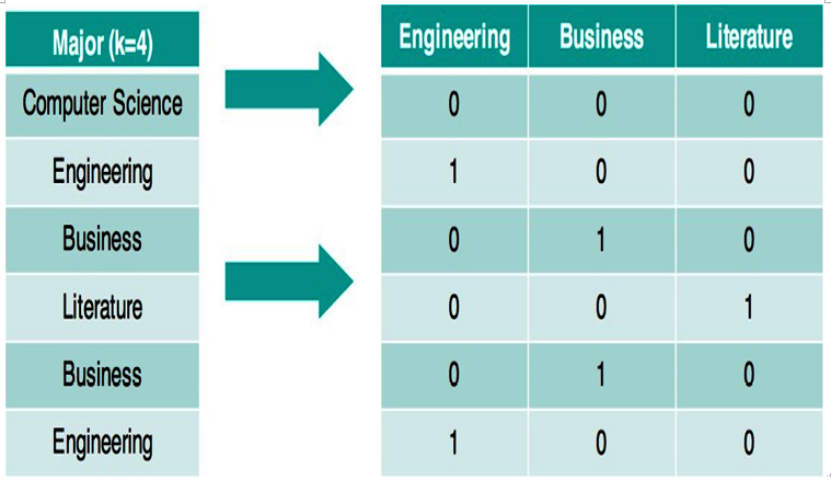
Figure 11.7 – Creating dummy variables for a single feature involves creating a new binary feature for each option except for one, which can be inferred by having all 0s in the rest of the features
Note that the first row has a 0 in all of the columns, which means that this person did not major in engineering, did not major in business, and did not major in literature. The second person has a single 1 in the Engineering column as that is the major they studied.
We are going to need to make some dummy variables using pandas as we use scikit-learn’s built-in decision tree function in order to build a decision tree:
# read in the data
titanic = pd.read_csv(‘short_titanic.csv’)
# encode female as 0 and male as 1
titanic[‘Sex’] = titanic.Sex.map({‘female’:0, ‘male’:1})
# fill in the missing values for age with the median age titanic.Age.fillna(titanic.Age.median(), inplace=True)
# create a DataFrame of dummy variables for Embarked
embarked_dummies = pd.get_dummies(titanic.Embarked, prefix=’Embarked’) embarked_dummies.drop(embarked_dummies.columns[0], axis=1, inplace=True)
# concatenate the original DataFrame and the dummy DataFrame titanic = pd.concat([titanic, embarked_dummies], axis=1)
# define X and y
feature_cols = [‘Pclass’, ‘Sex’, ‘Age’, ‘Embarked_Q’, ‘Embarked_S’] X = titanic[feature_cols]
y = titanic.Survived X.head()
Figure 11.8 shows what our dataset looks like after our preceding code block. Note that we are going to use class, sex, age, and dummy variables for city embarked as our features:
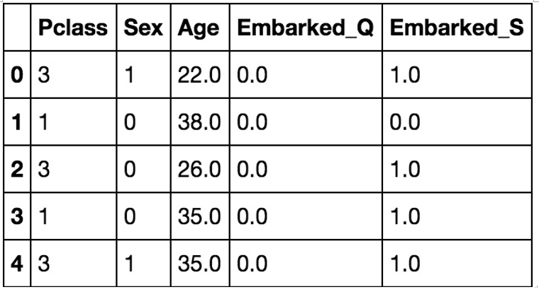
Figure 11.8 – Our Titanic dataset after creating dummy variables for Embarked
Now, we can fit our decision tree classifier:
# fit a classification tree with max_depth=3 on all data from sklearn.tree import DecisionTreeClassifier treeclf = DecisionTreeClassifier(max_depth=3, random_state=1) treeclf.fit(X, y)
max_depth is a hyperparameter that limits the depth of our tree. It means that, for any data point, our tree is only able to ask up to three questions and create three splits. We can output our tree into a visual format, and we will obtain the result seen in Figure 11.9:
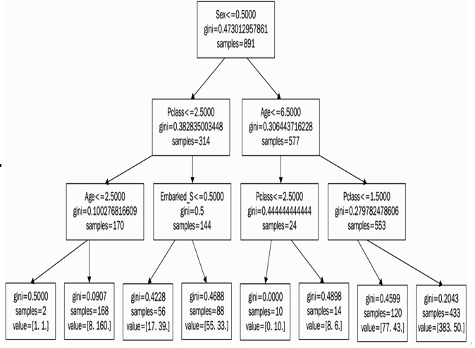
Figure 11.9 – The decision tree produced with scikit-learn with the Gini coefficient calculated at each node
We can notice a few things:
- Sex is the first split, meaning that sex is the most important determining factor of whether or not a person survived the crash
- Embarked_Q was never used in any split
For either classification or regression trees, we can also do something very interesting with decision trees, which is that we can output a number that represents each feature’s importance in the prediction of our data points (shown in Figure 11.10):
# compute the feature importances pd.DataFrame({‘feature’:feature_cols, ‘importance’:treeclf.feature_importances_})
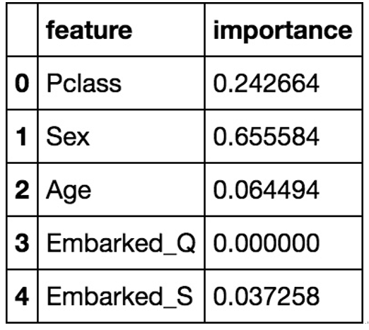
Figure 11.10 – Features that contributed most to the change in the Gini coefficient displayed as percentages adding up to 1; it’s no coincidence that our highest value (Sex) is also our first split
The importance scores are an average Gini index difference for each variable, with higher values corresponding to higher importance to the prediction. We can use this information to select fewer features in the future. For example, both of the embarked variables are very low in comparison to the rest of the features, so we may be able to say that they are not important in our prediction of life or death.
As we transition from the structured realm of SL, where the outcomes are known and the model learns from labeled data, we venture into the domain of UL. Recall that UL algorithms uncover hidden patterns and intrinsic structures within data that isn’t explicitly labeled. In the upcoming section, we will explore how unsupervised techniques can discern underlying relationships in data and provide deeper insights without the guidance of a predefined outcome, and how they can complement the predictive models we’ve discussed so far.